Notes: (1) Source: Penn World Tables; (2) For actual values, see Appendix A below; (3) GDP/worker is measured in constant 1985 "International Prices"
Gernot Köhler
School of Computing and Information Management
Sheridan College
Oakville, Ontario, Canada L6H 2L1
e-mail: gernot.kohler@sheridanc.on.ca
October 1999
1. SYNOPSIS
Neoclassical economists tend to be of the opinion that technological
progress is the main engine of worldwide economic growth. In
contrast, this study claims that technological progress is only a necessary,
not a sufficient condition for global income and output growth; and
that economic growth is also dependent on the growth of effective
demand, both nationally and within the world-system. The article discusses
Shaikh's isomorphism, explains it as a result of a Pasinetti-type
growth process, and applies these notions at the world level. According
to that view, long-term economic growth is driven by two "engines of growth",
not just one -- namely, by technological innovation (similar to Schumpeter's
notion) and by growth of effective demand (similar to Keynesian
notions). Inadequate growth of global demand in an environment of
global technological progress leads to economic growth rates below potential,
to income polarization, unemployment and underemployment. In other words,
whereas both supply constraints and demand constraints may exist in the
circular flow of the world economy (or a national economy), the growth
potential of the present world as a whole tends to be relatively more demand-constrained
than supply-constrained. This is explained in terms of a Pasinetti dynamic.
The institutions of world society must intervene in order to strengthen
the growth of global demand and improve its distribution, while supporting
technological innovation at the same time.
2. SCHUMPETER's COLD DOUCHE
Heilbroner writes in The Worldly Philosophers: "When he lectured
on the economy at Harvard in the midst of the depression, Joseph Schumpeter
would stride into the lecture hall, and divesting himself of his European
cloak, announce to the startled class in his Viennese accent, "Chentlemen,
you are vorried about the depression. You should not be. For capitalism,
a depression is a good cold douche." Having been one of those startled
listeners, I can testify that the great majority of us did not know that
a douche was a shower, but we did grasp that this was a very strange
and certainly un-Keynesian message." (Heilbroner 1986: 291) Rather than
rejecting either Schumpeter's or Keynes's theories, my strategy is to synthesize
the two points of view. This can be accomplished by using more recent theoretical
work by Shaikh, Felipe, McCombie, and Pasinetti. Given my interest in world-systems
research, I will develop my argument for both the national and the world-system
levels of analysis.
My presentation starts with a look at productivity growth. Two definitions
of productivity will be considered -- namely, "aggregate labour
productivity" (ALP, that is to say, GDP per worker; or, GDP per labour
hour) and "total factor productivity" (TFP; i.e., GDP per a weighted mix
of labour and capital inputs). Both concepts can be applied at the
national and world-system levels. I will not deal with the microeconomic
level. Ecological concerns must also be dealt with under the heading of
"global growth", but that is beyond this article.
3. PRODUCTIVITY GROWTH AND STANDARD OF LIVING
Productivity growth is correlated with the growth of the standard
of living of a community, but the relationship is neither automatic, nor
is aggregate productivity growth necessarily benefiting all members of
the community. In a polarized growth process, aggregate labour productivity
may rise, but there are winners and losers. While the winners may increase
their standard of living, the losers may have declining incomes at the
same time. In particular, productivity growth may be associated with increasing
unemployment. The productivity of the employed may increase, but
at the price of throwing others out of work through rationalization and
"downsizing", thus increasing unemployment.
4. ISOMORPHISM AND THE CRITIQUE OF "TOTAL FACTOR PRODUCTIVITY"
An important critique of neoclassical views of productivity growth has been developed by heterodox economists under the heading "isomorphism". Isomorphism of economic growth is a discovery by Shaikh (1974) and was further developed by Felipe (1998) and Felipe/McCombie (1998) and others. The criticism of this argument is directed against neoclassical production functions. A description of the neoclassical approach to the analysis of economic growth is, as follows: "Following Solow's study, it has been generally assumed that the whole economy (or sectors such as the private business sector or manufacturing) can be adequately described by a simple mathematical function such as: Q = F (L, K, t) where Q is value added, L is the labour input, K is the capital stock (adjusted for capital utilization) as a proxy for the flow of capital services, and t is time which supposedly captures exogenous technical change....Assuming neutral technical progress, the production function may be expressed as
Q = A(t) f(K,L)
[end quote]" (Felipe/McCombie 1998: 7). [In this formula, A(t) represents the notion of "level of technology at time t" ]
The heterodox critics have pointed out that this approach is isomorphic (tautological) with the national income side, as follows: "Following Shaikh, the accounting identity, which defines value added, is given by:
Qt = wt Lt + rt Kt
where Q, w, L, r, and K denote output (value added), the real wage, employment, the average rate of profit and the capital stock." (Felipe/McCombie 1998: 11-12)
Shaikh demonstrated that the two formulae above are formally equivalent (isomorphic). Based on the discovery of this formal equivalence between the two approaches to the analysis of economic growth and productivity growth, the heterodox authors have developed several points of critique, as follows. The heterodox critics acknowledge that neoclassical aggregate production functions tend to fit statistical time series quite well (empirical fit), but that they are weak, false or misleading in various other ways (theoretical misfit). The main criticisms can, perhaps, be listed, as follows: (1) There is a level-of-analysis problem: "Fisher ... demonstrated that the aggregate production function is not just a logical extension of the microeconomic production function" (Felipe/McCombie 1998: 35-36). (2) Problem with the concept of technology: "there is no such thing as the aggregate technology of a country, and therefore such idea cannot be represented in the so-called aggregate production function." (Felipe 1998: 19). (3) Problem with the measurement of technological change: TFP [sc. total factor productivity; used in econometric studies of aggregate production functions] is not necessarily a measure of technical change, but an "artifact" (Shaikh 1987); "the measure of TFP growth ...is not necessarily a measure of technical change ... one can never be certain that the coefficients estimated are the "true" technological parameters ... the same is true for growth accounting" (Felipe/McCombie 1998: 35-36). (4) Problem with explanatory power: the neoclassical aggregate production functions are based on "a law of algebra, not a law of production" and are "humbug" (Shaikh 1987: 690-1). Along the same line, Felipe (1998: 19) writes: "production functions can be interpreted as approximations to the said identity. As such, no behavioral content can be attached to them ... isomorphism between the production function and the value added accounting identity ... do not permit any inference about the alleged aggregate technology ... there is no such thing as the aggregate technology of a country, and therefore such idea cannot be represented in the so-called aggregate production function."
The above contributions are of a critical/deconstructive variety. Thus,
Felipe/McCombie (1998: 35-36) write: "We have neither provided new estimates
of TFP ... nor a new theory of growth..." In my humble opinion, Luigi Pasinetti
provides such an alternative theory of growth by making effective demand
an integral part of the economic growth process, along with technological
change.
5. PASINETTI ON GROWTH, TECHNOLOGY AND
EFFECTIVE DEMAND
While some heterodox economists were engaging in deconstruction of neoclassical
growth models -- e.g., Shaikh (1974, 1980), Felipe (1998) and Felipe/McCombie
(1998), Pasinetti engaged in construction of a post-Keynesian theory
of economic growth. Pasinetti's work is influenced by Schumpeter who coined
the phrase of capitalism as a process of "creative destruction". Both authors
have in common a belief in the importance of innovation. Both authors share
a broad, rather than narrow, concept of technological innovation, which
they view as a process of learning how to do things in new ways. This concept
of technological innovation goes beyond a narrow "hardware view" of technology
which equates technological progress with new machinery and gadgets and
nothing else. Thus, in the Schumpeter and Pasinetti view, a new operating
procedure or a new form of organization is as much eligible to be called
"technological innovation" as is a new type of computer hardware or a new
type of nuclear missile. Pasinetti considers technological progress, in
the sense of learning, as the major source of economic growth. Pasinetti
writes: "It is the acquisition of knowledge that eventually makes the wealth
of nations." (Pasinetti 1993: 176); and he describes technology as the
"primum movens" of economic growth (Pasinetti 1993: 45; "primum movens"
= primary moving force). This view of the importance of technological change
is similar to what we find in neoclassical theory of economic growth, e.g.,
in Robert Solow's work (Solow 1956, 1994). Where Pasinetti's theory differs
from the neoclassical one is regarding the role of effective demand.
Neoclassicals tend to ignore or deny a role for effective demand in the
process of economic growth or admit, at the most, that effective demand
plays a minor, short-term role (e.g., Mankiw, 1994). In contrast, Pasinetti's
theory assigns great importance to effective demand in long-term economic
growth. The argument runs, as follows: "Technical change emerges
as the crucial determinant in the dynamic process outlined by Pasinetti,
since it contains both a demand and a supply aspect." (Halevi 1994: 58).
In this process technological change propels both labour productivity and
per capita income simultaneously. However, there is no guarantee that there
will be a proper macroeconomic match between changing magnitudes of productivity
and changing magnitudes of aggregate income and demand. There is "no reliance
on any automatic fulfillment of the macroeconomic condition that ensures
the correct level of overall effective demand and hence full employment
" (Pasinetti 1993: 116). Technological progress and the growth of effective
demand are thus both needed for overall economic growth; one without the
other will not suffice. Thus, in the absence of sufficient effective demand,
"(t)echnological progress can ... also cause net losses of wealth or social
well-being in general" (Pasinetti 1993: 57). In Pasinetti's theory effective
demand co-determines the benefits reaped from technological progress, and
the institutions of society are seen as the guarantor who must assure that
effective demand and technological change are properly matched for
optimal social and economic results. Pasinetti's theory distinguishes between
a "physical quantity system" and a "price system" in the economy;
"(t)he physical quantity system is determined by the structural
evolution of consumption demand", while "(t)he price system
is determined by the structural evolution of technology" (Pasinetti
1993: 46; my emphasis). GDP (or, aggregate value added) is seen as the
sum of the cross-products of physical quantities and their prices. Thus,
demand determines one aspect of GDP and technology determines the other
aspect.
6. THREE CAUSAL VIEWS OF ISOMORPHISM
Isomorphism is not causation. The growth isomorphism described above can be interpreted in three different ways, depending on our postulates about causation, namely:
(1) neoclassical interpretation -- the supply side determines the income side, or,
A
f(K,L)
-- > Q
--> w L + r K
[read as causal arrows]
(engine of growth)
(passive)
(2) Shaikh's interpretation -- Q and incomes are determined by a "law of production"; the neoclassical side is "humbug", isomorphism is only a formal artifact; or,
A
f(K,L)
= Q
= w L + r K
(humbug,
^ ^ ^
^
[read as causal arrows]
artifact)
| | |
|
law of production
(3) Pasinetti-style interpretation -- the physical technology side and the effective demand side determine together, jointly and interactively, the value added (Q), or
A f(K,L) <--->
Q <--->
w L + r K
^
[read as causal arrows]
|
technological
demand
innovation
Pasinetti, like Schumpeter, takes innovation and technological change
seriously; and, like Kalecki, Keynes, Kaldor and Robinson, he takes effective
demand seriously. I find the combination of both elements in a theory
of economic growth (and productivity) very fruitful and will develop
my further presentation from this vantage point.
7. CIRCULATION OF VALUE IN THE ECONOMY
In order to understand the relationship between technology and effective
demand in the growth process, it is useful to examine the circular flow
of value in the economy. See Figure 7.1. This figure is very simple and
leaves out various important aspects of the circulation of value .)
FIGURE 7.1 CIRCULAR FLOW (without financial system, public sector,
international sector)
wL + rK
$----------------> INCOME------------->$
|
|
|
|
|
|
|
(money-
|
physical
E*P*f(K,L)
valued
|
production-------SUPPLY
circuit)
|
& technology
^
|
|
|
|
|
|
|
|
|
C + I
|
|
$< -----------------DEMAND <--------------$
|
|
goods & services,
|
commodities---------------
> --------- physical
(physical flow)
consumption &
investment
Note: for an explanation of the formulae, see the discussion in the
text
Figure 7.1 shows a circular flow (sorry, folks, the circle looks like a square, but imagine a circle!). In this circular flow, money (here "$") flows between three accounts -- namely, "INCOME", "DEMAND", and "SUPPLY" accounts. Since this is a circular flow, one cannot be sure where the circular flow started (another "chicken-and-egg" problem!). In order to underline the perpetual flow character, we could write, as follows:
[de infinito]-->income --> demand --> supply -->income --> demand --> supply --> income -->[ad infinitum]
Constraints in the circular flow may develop at any "transition stage", be it income, demand, supply or (here not elaborated:) additional money flows. Income dollars become demand dollars when the owner of the income decides to spend the income on purchases. Demand dollars become dollars in the producer/supplier's account when a purchase is made and paid for. The receipts from sales become payments to the factors of production, i.e., income of the factors "labour" and "capital".
Note that this refers to the circulation of monetary value, not physical
value. The physical objects and services (goods and services, commodities)
which correspond to the circulation of monetary value, are physically produced
on the supply side and and physically consumed on the demand side and circulate
physically from the producer/supplier side to the purchaser/demand side.
8. TWO DIMENSIONS OF AGGREGATE / SOCIETAL VALUE
There are two major dimensions of aggregate value in the circular flow
of the economy: (1) physical, (2) monetary. (Each of these can be subdivided.)
(1) Physical value: This is embodied in the physical objects
and services which are physically produced, sold and used. The measurement
of aggregate physical value leads to a listing of all physical goods and
services. The unit of measurement varies between items -- e.g., "pieces",
"tons", etc.
(2) Monetary value: This is the money value attached to the
physical values. The measurement of aggregate monetary value leads to
a single figure of aggregate value, expressed as monetary value (e.g.,
as GDP) -- unit of measurement =monetary (e.g., US $).
TABLE 8.1 EXAMPLE OF PHYSICAL AND MONEY-VALUED DIMENSIONS
Matrix
Matrix
Matrix
"Physical
"Unit price" "Group
Quantities"
Value"
(MOPh)
(MUP$)
(MGV$)
Description
shoes
10 pieces
20 $
200 $
steel
50 tons
200 $
10,000$
dentist
services 20 instances
70 $
140$
etc.
etc.
etc..
_________________________________________________
GDP (aggregate value added)[sum of above]
10,340 $
In short:
Aggregate value (AV$) = Sum (MGV$) = Sum (MOPh * MUP$)
= GDP$
The dual nature of aggregate value as physical value (things and actions)
and monetary value (dollars, etc.) is important for understanding the relationship
between technology and demand in the circular flow of the economy and in
economic growth (or decline) processes, because technology (including machinery
and know-how and organization) is physical ("real", as in a "thing"), whereas
demand is monetary.
9. TECHNOLOGY AND PHYSICAL VALUE
When we think strictly in physical terms, an increase in technological knowledge has the effect that more physical value can be produced with the same amount of physical input. For example, if, in a situation A, we have 10 workers (L=10) and 10 simple machines (KPh=10), we may be able to produce 200 shoes per hour (OPh = 200). The physical labour productivity in this situation is ALPPh=200/10=20 shoes per worker per hour. If technological sophistication increases, leading to a situation B, we may have 10 workers with higher skills and 10 sophisticated machines and may be able to produce 400 shoes per hour (OPh=400). The physical labour productivity is now ALPPh=400/10=40 shoes per worker per hour. Thus the increased technological sophistication had the effect of increasing physical output per hour and physical labour productivity. This "physical labour productivity" can also be called "physical labour efficiency". In this example, the efficiency of production in situation B is twice the physical efficiency in situation A. If we think strictly in terms of production, irrespective of sales and prices, it can be stated that, in the example, the doubling of physical efficiency had the effect of doubling the physical output.
Note that something very important is missing in this description
-- namely, there are no monetary values. There is no price information;
and there is no information about the total monetary value of the physical
output. We can describe an increase in aggregate physical value
in matrix form, as follows (Table 9.1):
TABLE 9.1
SITUATION A
SITUATION B
(with doubled physical efficiency)
Matrix
Matrix
"Physical
"Physical
Quantities"
Quantities"
(MOPh)
(MOPh)
Description Quantity
Description Quantity
shoes
10 pieces
shoes
20 pieces
steel
50 tons
steel
100 tons
dentist
dentist
services 20 instances
services 40
instances
etc.
etc.
In Table 9.1 physical output in Situation B is doubled in each category.
Note that we cannot say anything about prices and GDP (total monetary value
added), since we are strictly reasoning in physical terms. In this strictly
physical view, the physical output in Situation B (which is double that
in Situation A) cannot be summarized in a single number, because the units
of physical measurement vary from one category to the other. We have no
choice but to list the increased physical output by category (i.e., as
a matrix).
10. TECHNOLOGY AND THE TWO VALUE FORMS OF OUTPUT
This point is very important in my theory -- namely, that (1) aggregate output can be described in two alternate forms -- namely, in physical form, as a matrix of categories and their quantities; or, alternatively, in money-valued form, as a single figure which summarizes all the monetary values of all the categories [as shown in Table 8.1]; and that (2) technological knowledge has a direct influence on the physical efficiency of production, but has only an indirect influence on the monetary value of the output, since the aggregate monetary value of the physical output is a compound of both the physical output and prices. If, as in Table 8.1, the physical value of the physical output can be represented as a matrix (MOPh), which contains no monetary information, then the monetary value of this physical matrix can be arrived at by multiplying the various physical quantities by their unit prices. We thus multiply a physical matrix (MOPh) by a price matrix (MUP$). When the resulting cross-products are summed, we arrive at the monetary value of the aggregate output (AV$). The relationship between physical and monetary value of aggregate output is thus:
EQUATION 10.1
AV$ = Sum (MOPh * MUP$)
The differences between the two value forms of aggregate output can be described thus:
TABLE 10.1
AGGREGATE / SOCIETAL OUTPUT
PHYSICAL FORM MONEY-VALUED FORM
symbol in my examples
MOPh
AV$
full name of symbol
matrix of physical output
aggregate value in money terms
form of expression
matrix
single figure
content
physical
monetary
(goods, services)
unit(s) of measurement
tons, pieces, instances, etc.
dollar, yuan, etc.
usual names for this
none
GDP, or
(aggregate) value added, or
(aggregate) output
symbol for this, as
none
Y or Q or O
used in the literature
11. TWO DIMENSIONS OF AGGREGATE / SOCIETAL LABOUR PRODUCTIVITY
Parallel to the two value forms of aggregate output, there are two value forms of aggregate labour productivity -- namely, the physical and the money-valued form. The difference between physical and money-valued form of aggregate labour productivity results from the existence of the two forms of aggregate output (physical, monetary).
The physical form of aggregate labour productivity is in matrix notation (Equation 11.1):
EQUATION 11.1
MLPPh = MOPh / ML
in words, the matrix of physical labour productivity (MLPPh) is equal to the matrix of physical output (MOPh) divided by the matrix of volume of labour (ML). If I understand Pasinetti correctly, the rate of change of the various physical productivities contained in this matrix is called "rho" by Pasinetti (he uses the Greek letter). From this, Pasinetti calculates a weighted average rate of change of physical labour productivity, which he calls "rho*" (Pasinetti 1993: 70).
The money-valued form of aggregate labour productivity is a single figure, rather than a matrix (Equation 11.2):
EQUATION 11.2
ALP = AV$/L = Sum (MOPh * MUP$) / L
in words, aggregate labour productivity (ALP) is the quotient of aggregate
output in monetary form (AV$) divided by volume of labour (L).
The differences between the two value forms of aggregate labour productivity are:
TABLE 11.1
AGGREGATE / SOCIETAL LABOUR PRODUCTIVITY
PHYSICAL FORM MONEY-VALUED FORM
symbol in my equations
MLPPh
ALP
full name of symbol
matrix of physical labour
aggregate labour productivity
productivity
in money terms
form of expression
matrix
single figure
content
physical
monetary (for output)
(goods, services, jobs)
and physical (for labour)
unit(s) of measurement
tons, pieces, instances, etc.
dollar, yuan, etc.
and jobs (or labour hours)
and jobs (or labour hours)
usual names for this
none
(aggregate) labour productivity
symbol for this, as
none
Y/L or Q/L
used in the literature
other related terminology
rho and rho* (Pasinetti)
q for "net output per worker"
for growth rates of
(Shaikh) and q' for "growth rate
"labour productivity"
of net output per worker"
(physical)
(money-valued)
12. DOES THE NEOCLASSICAL PRODUCTION FUNCTION REPRESENT
PHYSICAL OR MONETARY VALUES?
Using the above definitions, we can make the following observations.
Observation 1: Equation 12.1 is true.
EQUATION 12.1
MOPh = MEPh * f (MKPh, MLPh)
[true]
or, in words, the matrix of physical output (MOPh) is equal to to the
product of a matrix of physical efficiency indexes times a function of
capital (K) and labour (L), understood as matrices of physical inputs.
This corresponds to my example in Table 9.1, where the efficiency index
for each category is assumed to be equal to 1.0 (in situation A)
and 2.0 (in situation B).
Observation 2: Equation 12.2 is false
EQUATION 12.2
AV$ = EPh * f (KPh, LPh)
[false]
or, in words, the monetary value of aggregate output (AV$) is equal
to the product of physical efficiency (EPh) times a function of capital
(K) and labour (L) inputs, understood as physical inputs.
The reason why this equation is false is that the left hand side of
the equation expresses monetary value, whereas all terms on the
right hand side express physical values. If we wanted to correct
this error, we would have to multiply the right hand side with a price
term of some kind.
Observation 3: The neoclassical production relation, as given by Solow (Equation 12.3), is problematic:
EQUATION 12.3
Q = A*f(K, L)
[problematic]
or, in words, aggregate output (Q) is equal to the product of level of technology (A) and a function of capital (K) and labour (L) inputs.
When we compare the three equations, the question arises whether Solow's
neoclassical equation is equivalent to my equation 12.1 (which is true)
or my equation 12.2 (which is false). My conclusion is that the neoclassical
function would be true, if it was interpreted in strictly physical
terms, as in my equation 12.1, where the letters symbolize matrices of
physical items. However, in neoclassical research practice, Solow's equation
is interpreted and operationally defined in mixed terms. In other
words, GDP is placed on the left hand side (this being a money-valued
term), while the terms on the right hand side are measured as (or,
are intended to be measures of) physical terms. This leads to a
gargantuan specification error in the research program of neoclassical
growth research, because the theoretical definition of the concepts does
not strictly correspond to the operational definitions of the concepts.
I concur with Shaikh, Felipe and McCombie therefore when they state that
the "Solow residual" (the "A" in Equation 12.3, or its growth form), as
measured in empirical studies, is not a true (unobtrusive) measure of the
(physical) level of technology but an "artifact" based on the isomorphism
with the national income accounting identity.
13. ISOMORPHISM BETWEEN INCOME AND DEMAND
Shaikh and others described an isomorphism between the (neoclassical) aggregate production function and the (heterodox) national income accounting identity (namely, Q = wL + rK; see above). It is reasonable to posit an additional isomorphism -- namely, an isomorphism between aggregate income and effective demand. This is based on familiar notions like a Keynesian consumption function, etc. Let C be aggregate consumption demand and I be aggregate (fixed-)investment demand (i.e., demand generated by capital expenditures). If aggregate consumption demand is some function of wage income and aggregate investment demand some function of capital incomes, we can write: C = f1(wL) and I = f2 (rK). If aggregate (effective) demand in the economy is AD, we arrive at a demand equation which is not identical with, but isomorphic with, the national income accounting identity -- namely Equation 13.1:
EQUATION 13.1
AD = C + I = f1(wL) + f2(rK)
where C is consumption demand and I is fixed-investment demand (also
called CAPEX in the literature), both including public and private components.
(This corresponds to the demand components D1 and D2 in Keynes's General
Theory.)
(Effective demand (AD) is a concept in the realm of monetary value,
rather than physical value. For example, effective demand in an economy
may be measured as 10 billion dollars at a particular time.)
14. DIFFERENCE BETWEEN PHYSICAL OUTPUT AND AGGREGATE SUPPLY
Aggregate supply (AS) is also a concept in the realm of monetary value, rather than physical value. For example, aggregate supply in an economy may be 10 billion dollars at a particular time. This figure does not reveal any information about physical quantities supplied. The missing link is price (more precisely, a matrix of unit prices). The relationship between physical output and aggregate supply can be stated as (Equation 14.1):
EQUATION 14.1
AS =Sum (MOPh * MUP$)
where AS is aggregate supply; MOPh is the matrix of physical output;
and MUP$ is the matrix of unit prices.
Note that aggregate supply is a money-valued concept.
15. GAINS AND LOSSES FROM TECHNOLOGICAL PROGRESS
The thesis of my study is that technological progress is only a necessary,
not a sufficient cause of economic growth. Economic growth is also
dependent on the growth of effective demand. This is in line with Pasinetti's
theory of economic growth. Pasinetti calls the growth process "structural
economic dynamics" (Pasinetti 1993, see title of book). The approach is
institutionalist, in the sense, that he calls his analysis "an inquiry
into the evolution of industrial systems" (Pasinetti 1993: 39). In
Pasinetti's theory "technological knowledge" and "learning" are seen as
the ultimate engine of growth. Thus, he describes his theory also as "a
theory of the economic consequences of learning" (Pasinetti 1993, see subtitle);
he describes technological progress as the "primum movens" (Pasinetti 1993:
45); and: "the acquisition of technological knowledge as the primary source
of the wealth of nations" (Pasinetti 1993: 174); and, again, in the last
sentence of his major study: "It is the acquisition of knowledge that eventually
makes the wealth of nations." (Pasinetti 1993: 176). We can see in this
the influence of Schumpeter. However, in addition to a need for Schumpeterian
innovation, Pasinetti diagnoses an equally important need for the growth
of effective demand. Effective demand growth must match (physical) technological
progress, or else a Marx/Keynes-type unemployment situation develops. There
is "no reliance on any automatic fulfillment of the macroeconomic condition
that ensures the correct level of overall effective demand and hence full
employment" (Pasinetti 1993: 116). If this condition is not met, "(t)echnological
progress can therefore -- through unemployment -- also cause net losses
of wealth and of social well-being in general" (Pasinetti 1993: 57).
15.1 LOSSES FROM TECHNOLOGICAL PROGRESS
Pasinetti's observation, namely, that a shortage of effective demand in an environment of technological progress may cause net losses of wealth and of social well-being, can be shown, as follows.
In ex-post analysis, the three magnitudes of GDP, aggregate supply and aggregate demand for a year are identical, namely:
EQUATION 15.1 [in ex-post analysis]
GDP = AS = AD
It follows, using my preceding equations and definitions, that:
EQUATION 15.2 [in ex-post analysis]
GDP = AS = Sum [MEPh * MUP$* f (MKPh, MLPh)]
= AD =
f1(wL) + f2(rK)
Let's simplify this by dropping the matrix notation, leading to:
EQUATION 15.3 [in ex-post analysis]
GDP = Q
= AS = E * P
* f(K, L)
[supply side]
= AD = f1(wL)
+ f2(rK)
[demand side]
in words, aggregate output (GDP) equals, on the supply side, an average weighted physical efficiency index derived from a matrix (E) times an average weighted supplier's price derived from a matrix (P) times a function of capital and labour inputs (K,L). Aggregate output (GDP) equals, on the demand side, consumption demand, which is a function of aggregate labour income (wL), plus fixed-investment demand, which is a function of aggregate capital income (rK). All this is in ex-post, static analysis.
This Equation 15.3 allows us to discuss some possible growth processes in a preliminary manner. Three kinds of possible losses from technological progress are (1) job losses (less L, more unemployment); (2) loss of labour income (less wL); (3) increased income polarization (the ratio rK/wL increases). Such losses could come about in Scenario 15.1:
SCENARIO 15.1 (technological progress with demand constraint)
(a) assume that physical technological efficiency increases (E increases)
(b) assume that aggregate demand cannot change (AD = constant), this
being a demand constraint
(c) assume that suppliers' selling prices do not change (P = constant)
What are some of the implications of this scenario, using Equation 15.3
for discussion? If aggregate demand is held constant, then (ex-post) aggregate
supply is constant as a result of the demand constraint (AS = AD). If,
as a consequence, aggregate supply is constant and suppliers' selling prices
are constant, then there are two expressions on the supply side which can
change (E and f(K,L)). We assume technological progress (E increases);
this forces the use of labour down (less L, more unemployment). What happens
on the demand side? We assumed that total effective demand is constant
(a demand constraint). Since there is a declining need for labour through
rationalization and down-sizing, there are also fewer workers on the demand
side. If wages are constant, there will be less effective demand from labour
since wL is decreasing. However, we said that aggregate demand remained
constant in this scenario. If total demand coming from labour declines
(less wL), then total demand from capital (rK) increases, in this scenario,
given the assumptions for this scenario. We thus have (1) technological
progress, with (2) constrained effective demand (both per assumption),
and, by implication, (3) more unemployment; (4) less total labour income;
and (5) more income polarization between labour and capital and more income
polarization between employed and unemployed labour. It is further noteworthy
that, in this scenario, decreasing employment (L) is accompanied by increasing
money-valued labour productivity (Q/L), since Q is constant and L is decreasing.
However, this increasing labour productivity does not make all of society
better off, since total output Q is constant in this scenario. For society
as a whole there is no gain from technological progress in this scenario.
15.2 GAINS FROM TECHNOLOGICAL PROGRESS
Our Equation 15.3 allows us also to discuss possible gains from
technological progress in a preliminary manner. Following Pasinetti, the
thesis of my study is that technological progress can bring gains for society,
but that these gains are conditional on parallel growth of effective demand.
Such gains could come about as in Scenario 15.2:
SCENARIO 15.2 (technological progress with adequate demand growth)
(a) assume that physical technological efficiency increases (E increases)
(b) assume that aggregate demand can change (AD = increasing), there
is no demand constraint
(c) assume that suppliers' selling prices do not change (P = constant)
What are some of the implications of this scenario 2, using Equation
15.3 for discussion? If aggregate demand increases in response to technological
progress, then all labour can remain employed (L = constant). With L and
P (suppliers' selling prices) being constant and technological efficiency
(E) increasing, total output (Q) increases. Since there is no demand constraint
in this scenario, demand increases commensurately with increasing supply
(as per assumption). Increasing demand implies that incomes for labour
(wK) and capital (rK) are rising. There is less pressure toward income
polarization than in Scenario 15.1 (with demand constraint). It is
further noteworthy that, in this scenario, aggregate labour productivity
(Q/L) is increasing, since Q is increasing and L is constant. Society as
a whole gains from technological progress in this scenario.
15.3 COMPARISON OF GAIN AND LOSS SCENARIOS
A comparison of the two scenarios above shows the crucial role of effective
demand in an environment of technological progress. Stagnant effective
demand, coupled with technological progress, leads to losses from
technological progress, including job losses, labour income losses and
increasing income polarization. In contrast, increasing effective demand,
coupled with technological progress, leads to gains from technological
progress (growth with less pressure toward unequal distribution). In both
scenarios aggregate labour productivity (Q/L) increases. However, the social
effects are significantly different. In the situation with stagnant
effective demand and with technological progress, increasing labour productivity
is coupled with increasing unemployment and no increase in aggregate income.
In contrast, in the situation with expanding effective demand and
technological progress, labour productivity increases as well, but employment
is steady and aggregate income increases.
16. TRANSFERABILITY TO THE WORLD-SYSTEM LEVEL
The concepts and inferences developed above in my theory section can also be applied at the world-system level. At the global level of analysis we treat the entire world economy as one organic whole (single system). My concepts and inferences were stated for "aggregates" and are equally applicable to "global aggregates". Thus we can re-write, for example, Equation 15.3 for the world-system level as Equation 16.1:
EQUATION 16.1 [in ex-post analysis]
World GDP
= Z
= GAS = E *
P * f(K, L)
[supply side]
= GAD = f1(wL)
+ f2(rK)
[demand side]
where
Z = world
product or world income
GAS = global aggregate supply
GAD = global aggregate demand
E = average weighted
global physical technological efficiency
P = average weighted
global suppliers' prices
K = volume of global
capital
L = volume of
global labour
w = global wage
level
r = global
rate of return on capital
In the same vain, the two definitions of (aggregate) labour productivity can be re-written from Equations 11.1 and 11.2 for the global level as Equations 16.2 and 16.3:
The physical form of global (aggregate) labour productivity is in matrix notation (Equation 16.2):
EQUATION 16.2
global MLPPh = global MOPh / global ML
in words, the matrix of physical labour productivity (MLPPh) is equal to the matrix of physical output (MOPh) divided by the matrix of volume of labour (ML), all with a global scope.
The money-valued form of global aggregate labour productivity is a single figure, rather than a matrix (Equation 16.3):
EQUATION 16.3
global ALP = Z/L
= global Sum (MOPh * MUP$) / L
in words, global aggregate labour productivity (ALP) is the quotient
of global product (Z) divided by global volume of labour (L), which is
also equal to the quotient of the global sum of all cross-products between
physical quantities and their unit prices, divided by volume of global
labour.
17. GLOBAL ISOMORPHISM
The isomorphism described by Shaikh and others, and the critique of
neoclassical growth theory derived from it, are also applicable at the
world-system level, since at the world level we deal with aggregates just
like at the national level. There is no difference in logic, if the world
system is treated as a single system. The main criticisms of neoclassical
aggregate production functions are also applicable at the world-system
level, namely: (1) there is a level-of-analysis problem (macro is not micro):
(2) there is a problem with the concept of technology; (3) there is a problem
with TFP [sc. total factor productivity]; it is an "artifact"
(Shaikh); (4) there is a problem with explanatory theory: neoclassical
aggregate production functions are based on "a law of algebra, not a law
of production" (Shaikh). (See also, section 4 above.)
18. GLOBAL GROWTH AS A PASINETTI PROCESS
I have argued above, along Pasinetti's lines, that technological progress
may propel growth of aggregate product and income, but that this result
is conditional on having sufficient growth of effective demand at the same
time. This thesis is also applicable at the world-system level, except
that at this level we speak of world income, global technological progress
and global effective demand, which must grow together in a matching way,
or else losses from global technological progress will ensue. These losses
from global technological progress may include (1) job losses in the world-system;
(2) stagnating world income; (3) increased global income polarization;
(4) increased intra-national income polarization. In a benign scenario
of global technological progress (i.e., with adequate growth of global
effective demand), global technological progress propels global labour
productivity and global aggregate income, without creating additional pressures
for global income polarization (or even with a reduction of global
income disparities). In a malignant scenario of global technological
progress (i.e., with stagnating global effective demand), global aggregate
labour productivity may also increase, but at the price of stagnating world
income, increasing world unemployment and worldwide income polarization.
(These statements are a transfer of corresponding statements from the national
level, in my theory sections above, to the world-system level.).
19. WORLD-SYSTEM AND NATIONAL PRODUCTIVITY
19.1 IN GENERAL
A number of interesting questions arise at the intersection between
world-system and national system. How does the world-system affect
national productivity? Is technological innovation a global, national,
or firm-level process? How do world market conditions affect national
productivity? and so on. My theory focuses on two concepts in particular,
which affect aggregate output -- namely, technological innovation and effective
demand. National economies are open to the world-system, especially to
the flow of information within the world-system. Technological know-how
is, on the one hand, guarded as company secrets and, on the other
hand, much of it spreads freely around the globe. There are imitation,
demonstration and catch-up effects, mingled with industrial espionage and
theft of intellectual property. National and company technological learning
is thus benefiting from a world-wide knowledge pool which influences
national productivity. Similarly, it can be observed that world
market conditions and global effective demand may have an impact
on national productivity. Here is an interesting example.
19.2 THE EXAMPLE OF SAUDI ARABIA
Saudi Arabia's productivity illustrates the influence of world
market conditions on national productivity. The development of Saudi Arabian
(aggregate) labour productivity is shown in Figure 1. (The data are from
Penn World Tables -- see also, Appendix A below.)
FIGURE 1. Saudi Arabia, Aggregate Labour Productivity, 1960 - 1989
Notes: (1) Source: Penn World Tables; (2) For actual values, see Appendix
A below; (3) GDP/worker is measured in constant 1985 "International Prices"
What explains the reversal of Saudi Arabia's (aggregate) labour productivity
after 1982? According to a common view, productivity growth is propelled
by technological progress (e.g., Solow) and/or improvement of "human capital"
(e.g., Mankiw) and other inputs. In the Saudi case, these explanations
appear inadequate for explaining the decline in aggregate productivity
after 1982; another explanation appears more plausible -- please examine
Figure 2.
FIGURE 2. Saudi Arabia -- GDP, Aggregate Labour Productivity and
Labour Force, 1960 - 1989
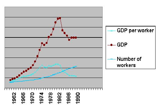
NOTES: (1) source: Penn World Tables; (2) for actual values,
see the table in Appendix A below; (3) GDP and GDP per worker measured
in constant 1985 "International Dollars" (PPP values)
Figure 2 shows that (1) the labour force (number of workers) increased steadily; (2) labour productivity (GDP per worker) first increased and then declined after 1982; and (3) GDP increased and, then, declined after 1982. There is a correlation between aggregate labour productivity (GDP per worker) and output (GDP).
The correlation between GDP and aggregate productivity
is not surprising, but causality requires some examination. It is
commonly assumed that variation in productivity (independent variable)
causes variation in output (dependent variable) [or, productivity --> output].
This assumption is not fully plausible in this case. If Saudi enterprises
and Saudi workers achieved a given level of technological sophistication
up to 1982, it is not plausible to assume that such sophistication suddenly
reversed itself after 1982. Another causal explanation is attractive --
namely, that the causation goes the other way, from GDP to productivity
(or, value of output --> value of productivity); in other words: after
1982, GDP declined and, therefore, aggregate labour productivity
declined. This view makes sense when we take world petroleum prices into
consideration. Petroleum is the major export of Saudi Arabia; and petroleum
revenue is a major component of Saudi GDP. When world oil prices
and world oil consumption increased, Saudi GDP increased handsomely.
When the world petroleum price declined in the 1980's, Saudi GDP slumped.
Saudi Arabian aggregate labour productivity declined concomitantly with
GDP.
The example of Saudi Arabia shows that the rise and fall of world prices
and world effective demand may induce a rise or fall of national GDP, which
may, in turn, induce a rise or fall in (national) aggregate (money-valued)
labour productivity. National aggregate labour productivity, as commonly
measured, may thus be a result of (a) world-system conditions, rather
than being of purely national origin; and/or (b) a result of demand-side
changes; there may thus ensue demand-pull productivity growth (or
decline), as opposed to supply-push productivity growth (or decline)
as in neoclassical theory.
20. TECHNOLOGICAL PROGRESS, EFFECTIVE DEMAND AND THE INSTITUTIONS
OF THE WORLD-SYSTEM
Pasinetti's theory of economic growth, with its dual emphasis on technological
innovation and effective demand, argues that the capitalist economic system
does not automatically bring about a proper match between growth of technological
efficiency and growth of effective demand. "This is the point where the
'institutional problems' ... become relevant." (Pasinetti 1993: 116) The
institutions of society must intervene in the market in order to bring
about the proper level of effective demand. Pasinetti speaks of the "existence
of a permanent task of pursuing ... effective demand and full employment"
(Pasinetti 1993: 59). I have argued above that economic growth at the world-system
level is a Pasinetti process of the same kind as that at the national (macroeconomic)
level. It can be claimed, therefore, that the institutions of the
world-system, as opposed to the market of the world-system, must
assure that the growth of effective demand in the world system is keeping
pace with technological progress. Under the heading of 'institutions of
the world system' we find many categories, including global and transnational
regulatory agencies like IMF, WTO, etc., corporate power structures, national
governments, non-governmental organizations and movements, and so on. A
recent topic of public debate has been "global financial architecture".
This and other global institutions need to be reformed or, if we talk about
labour and other citizens movements, then these movements need to assert
themselves, in order to strengthen, and improve the distribution
of, global effective demand and strengthen, and improve the distribution
of, the gains from global technological progress. According to the Universal
Declaration of Human Rights, everyone has an inalienable right to an adequate
standard of living.
21. REFERENCES
Felipe, Jesus (1998) "Singapore's Aggregate Production Function and its (Lack of) Policy Implications," Paper, e-mail of author: jfelipe@mail.asiandevbank.org
Felipe, Jesus, and JSL McCombie (1998) "Methodological Problems with Recent Analyses of the East Asian Miracle," Paper, e-mail of authors: jfelipe@mail.asiandevbank.org and jslm2@hermes.cam.ac.uk
Halevi, Joseph (1994) "Structure and Growth", Economie Appliquée, 1994, no. 2, 57 -80
Heilbroner, Robert L. (1986) The Worldly Philosophers. 6th ed. New York, USA: Simon & Schuster
Mankiw, N. Gregory (1994) Macroeconomics. 2nd edition. New York, USA: Worth Publishers
Pasinetti, Luigi L. (1993) Structural Economic Dynamics: A Theory of the Economic Consequences of Human Learning.
Penn World Tables (1999) at url: http://pwt.econ.upenn.edu
Shaikh, Anwar (1974) "Laws of Production and Laws of Algebra: The Humbug Production Function." The Review of Economics and Statistics, Vol. LVI, No. 61 (February): 115-20
Shaikh, Anwar (1987) "humbug production function", The New Palgrave (London, UK: MacMillan), Vol. 2, p. 690-692
Solow, Robert M. (1956) "A Contribution to the Theory of
Economic Growth," Quarterly Journal of Economics, Vol. 70, p. 65-94
22. RELATED PAPERS
Köhler, Gernot (1999) "Global Keynesianism and Beyond", Journal of World-Systems Research, https://jwsr.ucr.edu/ 5:225-241
Köhler, Gernot (1999) "A Theory of World Income",
World-Systems Archive, Working Papers, /archive/papers/kohler
23. APPENDIX A -- DATA FOR SAUDI ARABIA CASE
(see, Section 20.2)
Source: Penn World Tables
Notes: "International Prices" = term from Penn World Tables = purchasing
power parity dollars
"from
pwt" = from Penn World Tables
"my calc"
= my calculation from other data in the table
"RGDPL"
etc. are the variable names used in the Penn World Tables
|
Year
|
population
|
GDP per capita
|
GDP per worker
|
Number of workers
|
GDP
|
|
YEAR
|
POP
|
RGDPL
|
RGDPW
|
POP*RGDPL/RGDPW | POP* RGDPL |
|
from pwt
|
from pwt
|
from pwt
|
my calc
|
my calc | |
|
International prices
1985=100
|
International prices
1985=100
|
||||
|
1000s
|
1000s
|
billions | |||
|
1960
|
4075
|
3869
|
13798
|
1143
|
15.8
|
|
1961
|
4209
|
4238
|
15140
|
1178
|
17.8
|
|
1962
|
4348
|
4317
|
15459
|
1214
|
18.8
|
|
1963
|
4492
|
4851
|
17276
|
1261
|
21.8
|
|
1964
|
4640
|
5385
|
19315
|
1294
|
25.0
|
|
1965
|
4793
|
5981
|
21473
|
1335
|
28.7
|
|
1966
|
4970
|
6457
|
23200
|
1383
|
32.1
|
|
1967
|
5153
|
6612
|
23792
|
1432
|
34.1
|
|
1968
|
5343
|
6926
|
24949
|
1483
|
37.0
|
|
1969
|
5541
|
7151
|
25812
|
1535
|
39.6
|
|
1970
|
5745
|
7837
|
28345
|
1588
|
45.0
|
|
1971
|
5997
|
8755
|
31476
|
1668
|
52.5
|
|
1972
|
6275
|
9971
|
35625
|
1756
|
62.6
|
|
1973
|
6579
|
11445
|
40641
|
1853
|
75.3
|
|
1974
|
6905
|
12801
|
45195
|
1956
|
88.4
|
|
1975
|
7251
|
11714
|
41106
|
2066
|
84.9
|
|
1976
|
7617
|
11672
|
40730
|
2183
|
88.9
|
|
1977
|
8000
|
12549
|
43531
|
2306
|
100.4
|
|
1978
|
8410
|
12515
|
43131
|
2440
|
105.3
|
|
1979
|
8865
|
13130
|
45008
|
2586
|
116.4
|
|
1980
|
9372
|
13766
|
46849
|
2754
|
129.0
|
|
1981
|
9923
|
13779
|
46856
|
2918
|
136.7
|
|
1982
|
10510
|
13117
|
44608
|
3090
|
137.9
|
|
1983
|
11122
|
10214
|
34699
|
3274
|
113.6
|
|
1984
|
11750
|
9200
|
31216
|
3463
|
108.1
|
|
1985
|
12379
|
8313
|
28180
|
3652
|
102.9
|
|
1986
|
12991
|
7277
|
24716
|
3825
|
94.5
|
|
1987
|
13612
|
7300
|
24848
|
3999
|
99.4
|
|
1988
|
14016
|
7074
|
24128
|
4109
|
99.1
|
|
1989
|
14435
|
6876
|
23529
|
4218
|
99.3
|